What Actually Happens When You Calibrate a Weather Forecast

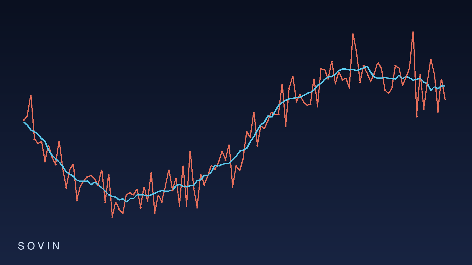
Calibrating a weather forecast means statistically correcting a numerical model’s known, repeatable errors using years of past forecasts compared against what actually happened. A raw physics model says the temperature at your local airport will be 34°C; the calibration layer knows that this particular model runs about 1.5 degrees too warm at that airport in calm summer conditions, and adjusts. The forecast you check on your phone is almost never raw model output — it’s model output after calibration.

This step is one of the quiet reasons forecasts have improved so much: alongside better physics and computing power, decades of statistical correction have been applied to every forecast you’ve ever seen.

Why Do Weather Models Need Correcting at All?

Numerical weather prediction (NWP) models divide the atmosphere into a grid and solve the equations of fluid dynamics and thermodynamics on it. They’re remarkable — but they have structural weaknesses that produce systematic errors, meaning errors that repeat in the same direction:

• Coarse resolution. A global model’s grid boxes might span 10–25 km. Your valley, coastline, or city heat island doesn’t exist at that scale.
• Approximated physics. Processes happening below grid scale — turbulence in the boundary layer, cloud microphysics, radiation through broken cloud — must be parameterized, i.e., approximated with simplified formulas. These approximations carry biases.
• Imperfect starting conditions. The atmosphere’s initial state is never known exactly, and small errors grow over the forecast.

The lowest layers of the model — the ones describing the air where people actually live — are generally the least faithful. Raw near-surface forecasts come out biased and noisy enough that forecasters historically wouldn’t use them directly.

Model Output Statistics (MOS): The Classic Method

The foundational fix dates to the late 1960s. Conceived within the U.S. National Weather Service’s Techniques Development Laboratory beginning in 1965, Model Output Statistics (MOS) produced its first operational forecasts in 1968, and Harry Glahn and Dale Lowry formally described the technique in their landmark 1972 paper.

The idea is simple and powerful:

1. Take an archive of past model forecasts for a location.
2. Pair each one with what actually happened there (the observations).
3. Run a multiple linear regression — with forward screening to pick the best predictors — relating the model’s forecast variables to the observed quantity you want, such as tomorrow’s maximum temperature or the probability of freezing precipitation.

The resulting equation implicitly absorbs everything the model can’t resolve: local terrain effects, known parameterization biases, seasonal behavior. NOAA’s Meteorological Development Laboratory, which still runs MOS today, feeds it three kinds of predictors: NWP model forecasts, prior observations, and geoclimatic data. MOS products based on the GFS and NAM models remain among the most-used guidance tools by National Weather Service forecasters.

A key advantage: because MOS is trained against reality, it can output genuinely reliable probabilities — “30% chance of rain” from MOS means rain occurred roughly 30% of the time in historical situations like this one. Raw single-run model output can’t honestly do that.

Calibrating Ensemble Forecasts

Modern forecasting leans on ensembles: instead of one forecast, run the model dozens of times with slightly different starting conditions. If most members agree, confidence is high; if they diverge, uncertainty is large. The spread of the ensemble is meant to estimate the probability of each outcome.

In practice, raw ensembles have a well-documented flaw: they’re typically underdispersed — the members cluster too tightly, meaning reality lands outside the ensemble envelope more often than it should. Treat the fraction of members predicting rain as “the chance of rain” and your probabilities won’t be reliable.

So ensembles get their own calibration, commonly via ensemble model output statistics (EMOS), also called nonhomogeneous Gaussian regression, introduced around 2005. Instead of a plain linear regression, EMOS fits the ensemble spread itself, learning how much to widen or narrow it so that, historically, the verified probabilities match the stated ones.

Forecasters diagnose whether an ensemble needs this treatment using tools like rank histograms: verify many ensemble forecasts, rank where the observation fell among the members, and plot the distribution. A flat histogram means well-calibrated; a U-shape means the observation falls outside the envelope too often — underdispersion; a hump means the ensemble is too spread out.

Where Machine Learning Fits In

The same logic now extends well beyond linear regression. Modern post-processing uses gradient-boosted trees, neural networks, and — since around 2023 — fully learned AI forecasting models such as ECMWF’s AIFS. Research published in Nature Communications Earth & Environment in 2021 showed that even low-cost statistical post-processing substantially improves skill globally, particularly for extreme rainfall.

The principle hasn’t changed since 1968: separate the model’s systematic error from the atmosphere’s genuine randomness, correct the first, quantify the second.

Does Calibration Actually Improve Forecasts?

Yes — measurably, and it compounds over time. ECMWF’s own analysis attributes its multi-decade skill gains partly to post-processing and data assimilation alongside model improvements; the widely cited figure is that medium-range forecast accuracy has improved by about one day per decade — today’s 5-day forecast is as accurate as a 4-day forecast was ten years ago. Post-processing studies consistently show bias-corrected, calibrated guidance beating raw model output, especially for surface quantities and extremes.

Frequently Asked Questions

What does it mean to calibrate a forecast?

To adjust a model’s output statistically so its errors — measured against long archives of past forecasts and observations — shrink, and so any stated probabilities match real-world frequencies.

What is Model Output Statistics (MOS)?

A technique defined by Glahn and Lowry in 1972 (operational in the U.S. since 1968) that uses multiple linear regression between archived numerical-model forecasts and actual observations to produce corrected, often probabilistic, forecasts of everyday weather quantities.

Why isn’t my weather app showing the raw model output?

Because raw near-surface output carries systematic biases from coarse grids and approximated physics. Statistical correction makes it both more accurate locally and honest about probabilities.

What is an underdispersed ensemble?

An ensemble whose members vary too little — reality falls outside the member spread more often than the probabilities imply. It signals overconfidence and is a prime target for spread-calibration methods like EMOS.

Do AI weather models need calibration too?

Yes. Learned models still exhibit systematic errors relative to observations, and probabilistic outputs still require reliability checks and correction before their numbers can be trusted the way calibrated MOS probabilities are.